

Performance Tuning
Most shove performance questions resolve to four levers: prefetch count, worker count, the concurrent-processing flag, and (negatively) transactional mode. Knowing which lever to pull first — and which to ignore — is what this page is for. The charts below are generated from a committed results document, and each carries its own provenance (shove version, generation date, hardware) in the caption; always measure on your own hardware and workload.
Benchmarks
Two conventions hold across every chart. A cell with no bar carries an explicit
n/s marker — never a zero, never a silently missing bar — and the chart's own
caption names why that cell has none: a window too short to publish as a rate, a
cell that failed to run, or a flow the backend cannot do at all (HasBroadcast /
HasCoordinatedGroups gate SQS's broadcast and consumer-group flows at compile
time). So n/s on its own does not mean "not supported"; the note beside it says
which of those it is. And a backend the results document does not contain is
never plotted, so absence from a chart means "not measured here", not "slow".
The document these charts render from measures all six backends: in-process, Kafka, NATS, RabbitMQ, Redis and SQS. The SQS rows measure LocalStack, which is non-representative of the AWS service by design, and run a smaller corpus than the other backends; the rows and the charts record both (see the benchmark runbook's "The SQS corpus deviation"). Every run was measured on the same host: the harness refuses to merge runs from different hosts into one document.
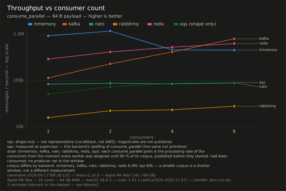
Throughput vs consumer count
How drain rate scales with consumer count, per backend.
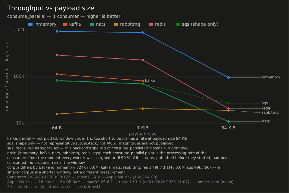
Throughput vs payload size
The cost of moving 64 B, 1 KiB and 64 KiB messages through the same flow.
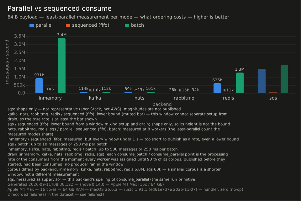
Parallel vs sequenced
What ordering costs: the same workload consumed in parallel and through sequenced (FIFO) delivery.
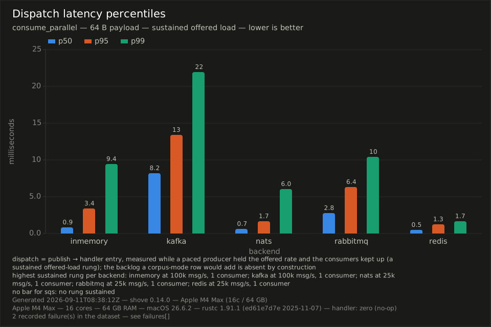
Dispatch latency
Per-message dispatch percentiles (p50/p95/p99). When the results document cannot support the claim, the chart refuses on its face instead of plotting a misleading number — the accounting for each backend is rendered in the chart itself.
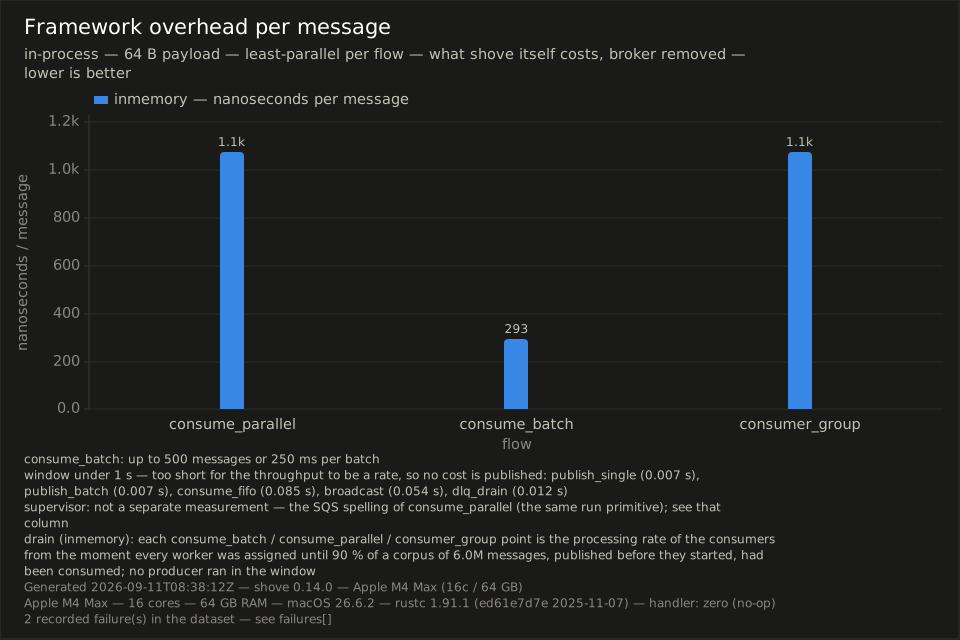
Framework overhead
What shove itself costs, in nanoseconds per message per flow — measured on the in-process backend so no broker round-trip is included.
The throughput levers
In order of impact:
prefetch_count(largest lever): how many unacked messages the broker pre-delivers to a consumer. Higher values mean more in-flight work and fewer round-trips waiting for acks.- Worker count (linear scaling on handler-bound workloads): more concurrent handlers means more throughput when handlers are CPU- or I/O-bound. Scaling is close to linear until you hit a broker or partition limit.
concurrent_processingflag:trueallows multiple handler invocations to run concurrently within a single worker, bounded byprefetch_count.false(default) processes one message at a time per worker.- Transactional mode (negative lever): the
rabbitmq-transactionalfeature reduces throughput roughly 10–15× per channel compared to non-transactional. The trade-off is routing safety — every ack and publish land in the same AMQP transaction.
Batching and payload size. BatchConsumer amortises one handler call over
max_batch_size messages, and that pays when the per-message cost is the
handler call itself. It stops paying as the payload grows. Comparing the
in-process batch drain against the plain parallel drain at the same cell, the
committed document has the batch flow at 3.6-9.7x the parallel rate at 64 B,
0.9-3.1x at 1 KiB and 0.5-1.2x at 64 KiB — so what turns the comparison
around is payload size, and by 64 KiB batching is a wash at best: only the
eight-consumer cell is above parity there, and the single-consumer one runs at
about half the parallel rate. Every bound is rounded outward, so no drain row
falls outside a range stated here. One cell behind these ranges is in the
document but not on the charts — the 64 B two-consumer batch drain finished
under the harness's reliability floor and is withheld with an n/s marker;
every 64 KiB drain row publishes. Batch small messages; consume large ones one
at a time.
prefetch_count deep-dive
prefetch_count tells the broker how many unacked messages it may deliver to a single consumer before waiting for acks. With prefetch_count = 1, the broker waits for an ack before sending the next message — every handler invocation pays a full network round-trip. With higher values, the consumer has a local buffer of pre-delivered messages and can begin processing the next one immediately after finishing the previous.
Why too high is also a problem: if one consumer holds a large unacked backlog, other consumers in the same group receive less work — distribution becomes uneven. Very high values also increase per-consumer memory usage and slow graceful shutdown (all unacked messages must drain).
Recommended starting point: 10–40. Tune based on handler latency: short-latency handlers benefit more from high prefetch; long-latency handlers (where the bottleneck is the handler itself) need high worker counts instead.
Worked example. Handler average latency 10 ms, network RTT 1 ms:
prefetch_count = 1: every message pays the full 11 ms cycle — 10 ms of handler work plus a round-trip idle waiting for the next delivery. The round-trip tax caps throughput below what the handler alone could sustain.prefetch_count = 20: the consumer always has the next message buffered, so the cycle is the 10 ms of handler work — the handler runs at close to its own maximum rate.
Workers — when to add them
Add workers when the topic backlog grows faster than the consumer drains it. That's the signal that the handler is the bottleneck.
A single shove consumer rarely saturates the network or broker on its own. The bottleneck is almost always handler latency × concurrency. Each additional worker adds a parallel handler goroutine; throughput scales linearly until you hit:
- Broker quota — e.g. RabbitMQ per-connection channel limits.
- Partition count (Kafka) — a 4-partition topic can only be consumed by 4 group members simultaneously.
- Sub-queue count (RabbitMQ sequenced) — the number of consistent-hash shards limits sequenced consumer parallelism.
with_concurrent_processing(true)
When concurrent_processing is true, a single worker can have multiple handler invocations in-flight simultaneously, limited by prefetch_count. The benefit is full utilization of the pre-fetched buffer: while one handler is awaiting a database response, another can start.
Use when: handlers are pure I/O-bound — waiting on a database query, an HTTP call, an external API. The async runtime multiplexes tasks efficiently.
Don't use when: handlers are CPU-bound. Concurrent tasks without additional OS threads don't add parallelism — they compete for the same thread pool and can increase latency without improving throughput. For CPU-bound work, increase worker count instead.
Measurement methodology
The published charts render from a committed results document,
benches/results/bench-results.json, measured one backend at a time. Every
published row comes from the same pinned matrix, and that matrix lives in
exactly one place — the MATRIX array in scripts/bench.sh — so a run is
reproduced by invoking the script per backend, not by assembling the flags by
hand:
scripts/bench.sh inmemory --fresh # then kafka, nats, rabbitmq, redis
dotenvx run -- scripts/bench.sh sqsThe script picks each backend's example target and feature flag (the full table
is in Choosing a backend), checks the prerequisites, tees
the harness output into target/bench-logs/, and merges the run into the
document by backend key. On your own hardware the first backend needs --fresh,
as above: the harness refuses to merge a run into a document measured on a
different host, toolchain or crate version, so one document is always one host.
Beyond the (flow, payload, tier, handler, consumers) sweep, the matrix pins
how the consume flows are measured, which is what the throughput and latency
charts read respectively: a drain of a corpus published before any consumer
starts, which is the throughput ceiling, and a paced offered-load ladder,
which is where the dispatch-latency percentiles come from. Every row of those
flows records which under method. The harness stamps provenance — shove
version, generation date, hardware, toolchain — into the document, and every
chart caption renders it. The per-backend deviations from that matrix, and how
to read a finished run, are in the
benchmark runbook.
The charts regenerate from the committed document, and the same script runs the byte-compare CI enforces:
scripts/bench.sh charts
# what it runs, if you want the renderer alone
cargo run --no-default-features --example chartgen -- \
--input benches/results/bench-results.json --out-dir docs/public/benchtests/chartgen.rs byte-compares the committed SVGs against the committed
results document, so a results file updated without regenerating the charts —
or a hand-edited chart — fails the test suite.
Hardware, broker version, network setup, and OS scheduler all affect results. The charts are a starting reference — measure on your own setup before committing to a configuration.
What NOT to tune first
Ranked by typical impact:
- Serde format — JSON serialization overhead is negligible compared to network round-trip. Switching to bincode or MessagePack rarely moves the needle for normal message sizes.
- Connection pool size — a single AMQP channel or Kafka producer moves messages far faster than a typical handler consumes them. Pooling is for fault-tolerance (connection failover), not raw throughput.
- TLS — modern TLS handshake and record overhead is negligible for the message sizes and rates shove handles. Disable only if profiling shows it in a hot path.
- Tracing — structured logging at
infolevel adds less than 1% overhead. Disable only atdebuglevel if profiling shows it dominates.
What's next
- Backend Ops Notes — per-backend production knobs and gotchas
- Consumer Groups & Autoscaling — autoscaler configuration and scaling policies
- RabbitMQ stress example — walk through the benchmark harness